Terms
Because a relation is a mathematical construct, end users find it much easier to think of a relation as a table. A table is perceived as a two-dimensional structure composed of rows and columns. A table is also called relation.
1. A table is perceived as a two-dimensional structure composed of rows and columns.
2. Each table row (tuple) represents a single entity occurrence within the entity set.
3. Each table column represents an attribute, and each column has a distinct name.
4. Each intersection of a row and column represents a single data value.
5. All values in a column must conform to the same data format.
6. Each column has a specific range of values known as the attribute domain.
7. The order of the rows and columns is immaterial to the DBMS.
8. Each table must have an attribute or combination of attributes that uniquely identifies each row, primary key(PK).
Keys: A key consists of one or more attributes that determine other attributes.
Determination is the state in which knowing the value of one attribute makes it possible to determine the value of another. Determination in a database environment, however, is not normally based on a formula but on the relationships among the attributes.
functional dependence means that the value of one or more attributes determines the value of one or more other attributes.
In this functional dependency, the attribute whose value determines another is called the determinant or the key. The attribute whose value is determined by the other attribute is called the dependent.
- A superkey is a key that can uniquely identify any row in the table.
- A candidate key is a minimal superkey—that is, a superkey without any unnecessary attributes.
Entity integrity is the condition in which each row (entity instance) in the table has its own unique identity.
To ensure entity integrity, the primary key has two requirements:
(1) all of the values in the primary key must be unique,
(2) no key attribute in the primary key can contain a null.
A null is the absence of any data value, and it is never allowed in any part of the primary key.
- a table that contains a null is not properly a relational table at all.
- In fact, an abundance of nulls is often a sign of a poor design.
A foreign key (FK) is the primary key of one table that has been placed into another table to create a common attribute.
Foreign keys are used to ensure referential integrity, the condition in which every reference to an entity instance by another entity instance is valid. In other words, every foreign key entry must either be null or a valid value in the primary key of the related table.
Secondary key is defined as a key that is used strictly for data retrieval purposes. Keep in mind that a secondary key does not necessarily yield a unique outcome.
Integrity rules
- Entity integrity
- Referential integrity
To avoid nulls, some designers use special codes, known as flags, to indicate the absence of some value.
Other solution includes NOT NULL and UNIQUE.
The NOT NULL constraint can be placed on a column to ensure that every row in the table has a value for that column. The UNIQUE constraint is a restriction placed on a column to ensure that no duplicate values exist for that column.
Relational algebra
Relational algebra defines the theoretical way of manipulating table contents using relational operators.
A relation is the data that we see in our tables. A relvar is a variable that holds a relation.
A relvar has two parts: the heading and the body. The relvar heading contains the names of the attributes, while the relvar body contains the relation. To conveniently maintain this distinction in formulas, an unspecified relation is often assigned a lowercase letter (e.g., “r”), while the relvar is assigned an uppercase letter (e.g., “R”). We could
then say that r is a relation of type R, or r(R).
The relational operators have the property of closure; that is, the use of relational algebra operators on existing relations (tables) produces new relations.
select (σ)
Select (Restrict) SELECT, also known as RESTRICT, is referred to as a unary operator because it only uses one table as input. It yields values for all rows found in the
table that satisfy a given condition. SELECT can be used to list all of the rows, or it can yield only rows that match a specified criterion.
SELECT is denoted by the lowercase Greek letter sigma (σ). Sigma is followed by the condition to be evaluated (called a predicate) as a subscript, and then the relation is
listed in parentheses.
For example, to SELECT all of the rows in the CUSTOMER table that have the value ‘10010’ in the CUS_CODE attribute, you would write the following:
Project (π)
PROJECT yields all values for selected attributes. It is also a unary operator, accepting only one table as input. PROJECT will return only the attributes requested,
in the order in which they are requested. In other words, PROJECT yields a vertical subset of a table.
Formally, PROJECT is denoted by the Greek letter pi (π). For example, to PROJECT the CUS_FNAME and CUS_LNAME attributes in the CUSTOMER table, you would write the following:
Union (∪)
UNION combines all rows from two tables, excluding duplicate rows. To be used in the UNION, the tables must have the same attribute characteristics; in other words, the columns and domains must be compatible. When two or more tables share the same number of columns, and when their corresponding columns share the same or compatible domains, they are said to be union-compatible.
For example, assume the SUPPLIER and VENDOR tables are not union-compatible. If you wish to produce a listing of all vendor and supplier names, then you can PROJECT the names from each table and then perform a UNION with them.
Intersect (∩)
INTERSECT yields only the rows that appear in both tables.
For example, again assume the SUPPLIER and VENDOR tables are not union-compatible. If you wish to produce a listing of any vendor and supplier names that are the same in both tables, then you can PROJECT the names from each table and then perform an INTERSECT with them.
Difference
DIFFERENCE yields all rows in one table that are not found in the other table; that is, it subtracts one table from the other. As with UNION, the tables must be union-compatible to yield valid results. However, note that subtracting the first table from the second table is not the same as subtracting the second table from the first table.
DIFFERENCE is denoted by the minus symbol −. If the relations SUPPLIER and VENDOR are union-compatible, then an DIFFERENCE of SUPPLIER minus VENDOR would be written as follows:
supplier − vendor
Assuming the SUPPLIER and VENDOR tables are not union-compatible, producing a list of any supplier names that do not appear as vendor names, then you can use a DIFFERENCE operator.
Product
PRODUCT yields all possible pairs of rows from two tables—also known as the Cartesian product. Therefore, if one table has 6 rows and the other table has 3 rows,
the PRODUCT yields a list composed of 6 × 3 = 18rows.
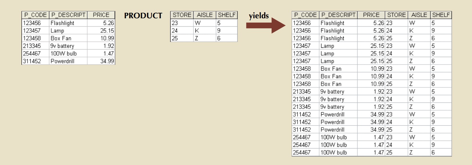
PRODUCT is denoted by the multiplication symbol ×. The PRODUCT of the CUSTOMER and AGENT relations would be written as follows:
customer × agent
Join
JOIN allows information to be intelligently combined from two or more tables.
JOIN is the real power behind the relational database, allowing the use of independent tables linked by common attributes.
Natural Join ( )
)
A natural join links tables by selecting only the rows with common values in their common attribute(s). A natural join is the result of a three-stage process:
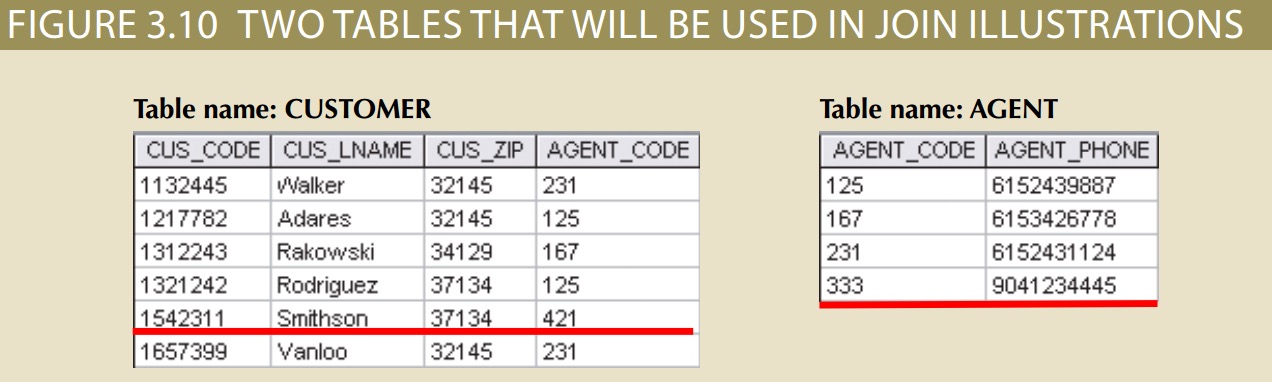
1. First, a PRODUCT of the tables is created, yielding the results shown in Figure.
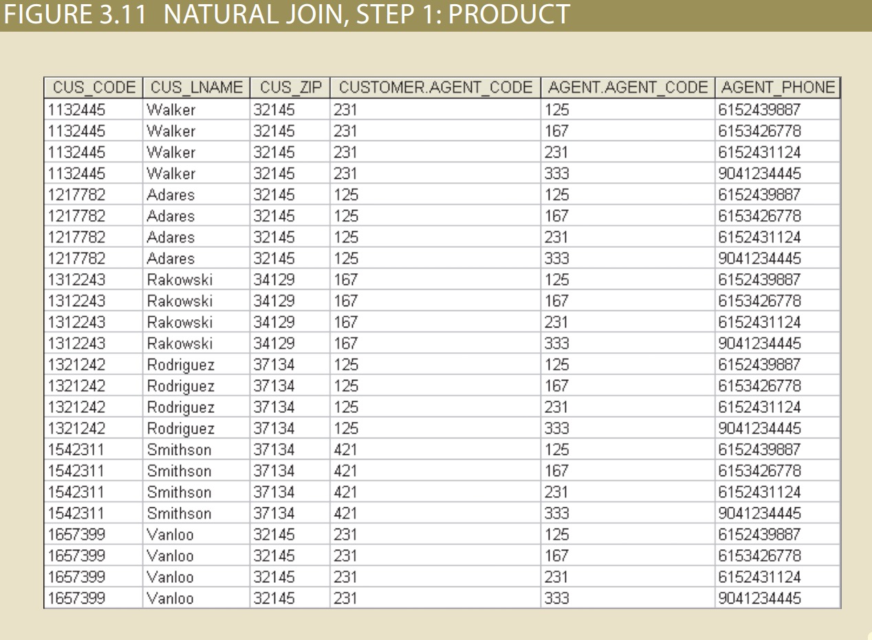
2. Second, a SELECT is performed on the output of Step 1 to yield only the rows for which the AGENT_CODE values are equal. The common columns are referred to as the join columns. Step 2 yields the results shown in Figure 3.12.
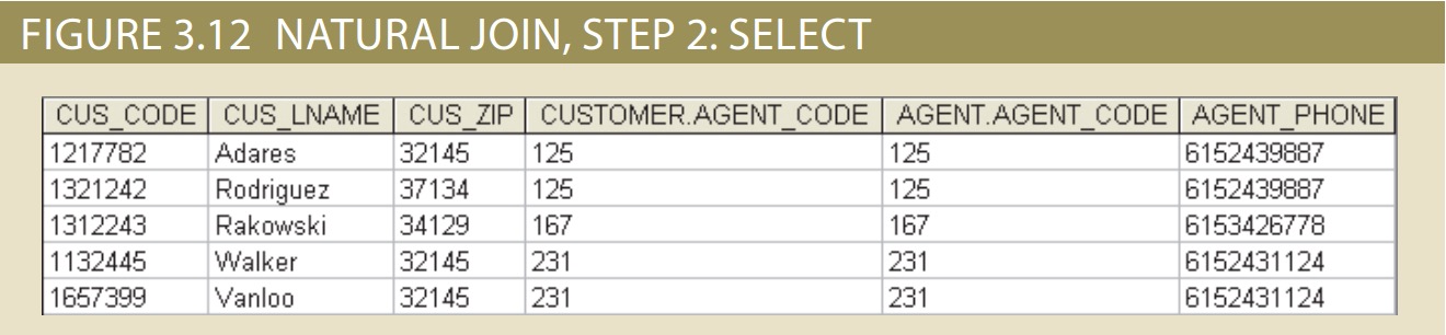
3. A PROJECT is performed on the results of Step 2 to yield a single copy of each attribute, thereby eliminating duplicate columns. Step 3 yields the output shown
in Figure 3.13.
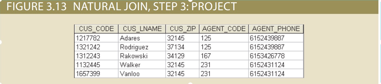
The final outcome of a natural join yields a table that does not include unmatched pairs and provides only the copies of the matches.
Note a few crucial features of the natural join operation:
• If no match is made between the table rows, the new table does not include the unmatched row. In that case, neither AGENT_CODE 421 nor the customer whose
last name is Smithson is included. Smithson’s AGENT_CODE 421 does not match any entry in the AGENT table.
• The column on which the join was made—that is, AGENT_CODE—occurs only once in the new table.
• If the same AGENT_CODE were to occur several times in the AGENT table, a customer would be listed for each match. For example, if the AGENT_CODE 167 occurred three times in the AGENT table, the customer named Rakowski would also occur three times in the resulting table because Rakowski is associated with AGENT_CODE 167. (Of course, a good AGENT table cannot yield such a result because it would contain unique primary key values.)
Natural join is normally just referred to as JOIN in formal treatments. JOIN is denoted by the symbol ⨝. The JOIN of the CUSTOMER and AGENT relations would be written as follows:
customer ⨝ agent
Notice that the JOIN of two relations returns all of the attributes of both relations, except only one copy of the common attribute is returned. Formally, this is described as a UNION of the relvar headings. Therefore, the JOIN of the relations (c ⨝ a) includes the UNION of the relvars (C ∪ A). Also note that, as described above, JOIN is not a fundamental relational algebra operator. It can be derived from other operators as follows:
Equijoin (  )
)
Another form of join, known as an equijoin, links tables on the basis of an equality condition that compares specified columns of each table. The outcome of the equijoin does
not eliminate duplicate columns, and the condition or criterion used to join the tables must be explicitly defined. In fact, the result of an equijoin looks just like the outcome
shown in Figure 3.12 for Step 2 of a natural join. The equijoin takes its name from the equality comparison operator (=) used in the condition. If any other comparison operator is used, the join is called a theta join.
In formal terms, theta join is considered an extension of natural join. Theta join is denoted by adding a theta subscript after the JOIN symbol: ⨝θ. Equijoin is then a special type of theta join.
Each of the preceding joins is often classified as an inner join. An inner join only returns matched records from the tables that are being joined.
Outerjoin
In an outer join, the matched pairs would be retained, and any unmatched values in the other table would be left null. It is an easy mistake to think that an outer join is the opposite of an inner join.
However, it is more accurate to think of an outer join as an “inner join plus.” The outer join still returns all of the matched records that the inner join returns, plus it returns the unmatched records from one of the tables. More specifically, if an outer join is produced for tables CUSTOMER and AGENT, two scenarios are possible:
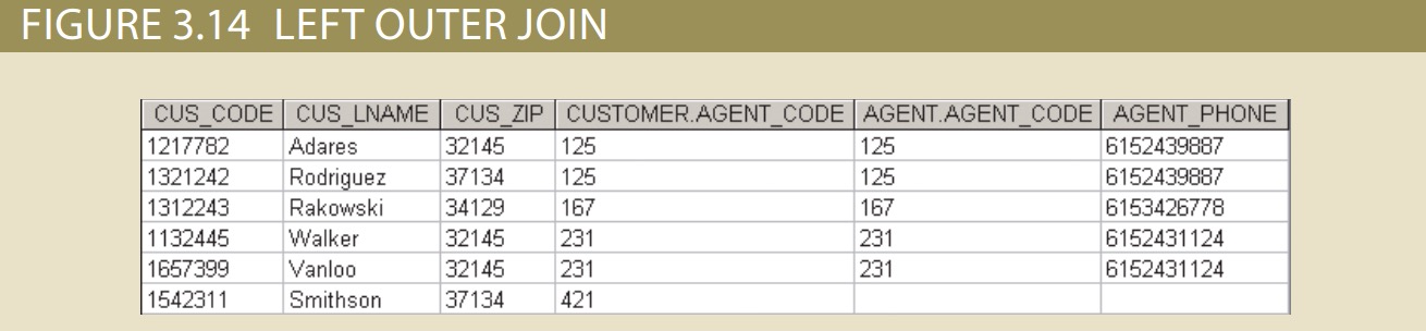
A left outer join yields all of the rows in the CUSTOMER table, including those that do not have a matching value in the AGENT table. An example of such a join is shown
in Figure 3.14.
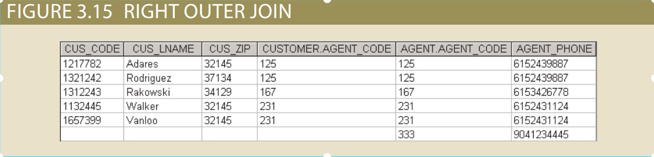
• A right outer join yields all of the rows in the AGENT table, including those that do not have matching values in the CUSTOMER table. An example of such a join is shown in Figure 3.15.
Outer joins are especially useful when you are trying to determine what values in related tables cause referential integrity problems. Such problems are created when foreign
key values do not match the primary key values in the related table(s). In fact, if you are asked to convert large spreadsheets or other “nondatabase” data into relational database.
You may wonder why the outer joins are labeled “left” and “right.” The labels refer to the order in which the tables are listed in the SQL command. Left and right outer joins are denoted by the symbols ⟕ and ⟖, respectively.
Divide (÷)
The DIVIDE operator is used to answer questions about one set of data being associated with all values of data in another set of data. The DIVIDE operation uses one
2-column table (Table 1) as the dividend and one single-column table (Table 2) as the divisor.
For example, Figure 3.16 shows a list of customers and the products purchased in Table 1 on the left. Table 2 in the center contains a set of products that are of interest to
the users. A DIVIDE operation can be used to determine which customers, if any, purchased every product shown in Table 2.
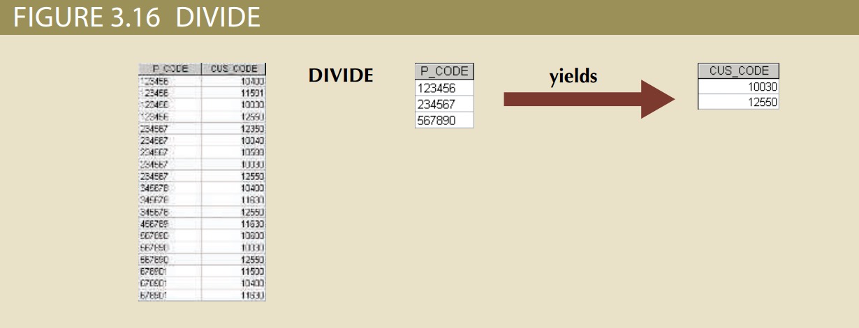
• Table 1 is “divided” by Table 2 to produce Table 3. Tables 1 and 2 both contain the P_CODE column but do not share the CUS_CODE column.
• To be included in the resulting Table 3, a value in the unshared column (CUS_CODE) must be associated with every value in Table 2.
• The only customers associated with all of products 123456, 234567, and 567890 are customers 10030 and 12550.
The DIVIDE operator is denoted by the division symbol ÷. Given two relations, R and S, the DIVISION of them would be written: r ÷ s.
The Data Dictionary and the System Catalog
The data dictionary contains metadata—data about data.
The DBMS’s internally stored data dictionary contains additional information about relationship types, entity and referential integrity checks and enforcement, and
index types and components. This additional information is generated during the database implementation stage. The data dictionary is sometimes described as “the database designer’s database” because it records the design decisions about tables and their structures.
The system catalog can be described as a detailed system data dictionary that describes all objects within the database, including data about table names, table’s creator and creation date, number of columns in each table, data type corresponding to each column, index filenames, index creators, authorized users, and access privileges.
In fact, current relational database software generally provides only a system catalog. In a database context, the word homonym indicates the use of the same name to label different attributes. For example, you might use C_NAME to label a customer name attribute in a CUSTOMER table and use C_NAME to label a consultant name attribute in a CONSULTANT table. To lessen confusion, you should avoid database homonym. a synonym is the opposite of a homonym, and indicates the use of different names to describe the same attribute. For example, car and auto refer to the same object. Synonyms must be avoided whenever possible.
Database relation
1:M, 1:1, M:N three relation can be implemented:
• The 1:M relationship is the relational modeling ideal. Therefore, this relationship type should be the norm in any relational database design.
• The 1:1 relationship should be rare in any relational database design.
• M:N relationships cannot be implemented as such in the relational model.
1:M relation
The one-to-many (1:M) relationship is easily implemented in the relational model by putting the primary key of the “1” side in the table of the “many” side as a foreign key.
consider the PAINTER and PAINTING example:

As you examine the PAINTER and PAINTING table contents in Figure 3.18, note the following features:
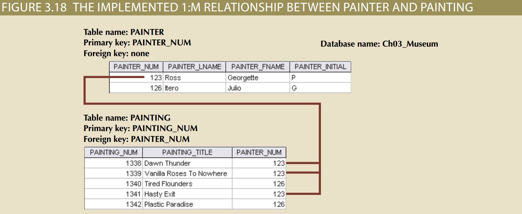
• Each painting was created by one and only one painter, but each painter could have created many paintings. Note that painter 123 (Georgette P. Ross) has three works
stored in the PAINTING table.
• There is only one row in the PAINTER table for any given row in the PAINTING table, but there may be many rows in the PAINTING table for any given row in the PAINTER table.
The 1:1 Relationship
As the 1:1 label implies, one entity in a 1:1 relationship can be related to only one other entity, and vice versa. For example, one department chair—a professor—can chair only one department, and one department can have only one department chair.
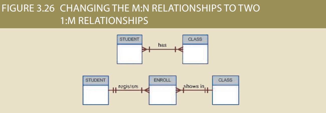
The M:N Relationship
A many-to-many (M:N) relationship is not supported directly in the relational environment. However, M:N relationships can be implemented by creating a new entity in 1:M
relationships with the original entities. To explore the many-to-many relationship, consider a typical college environment.
The ER model in Figure 3.23 shows this M:N relationship:

Fortunately, the problems inherent in the many-to-many relationship can easily be avoided by creating a composite entity (also referred to as a bridge entity or an
associative entity). Because such a table is used to link the tables that were originally related in an M:N relationship, the composite entity structure includes—as foreign keys—at least the primary keys of the tables that are to be linked. The database designer has two main options when defining a composite table’s primary key: use the
combination of those foreign keys or create a new primary key.
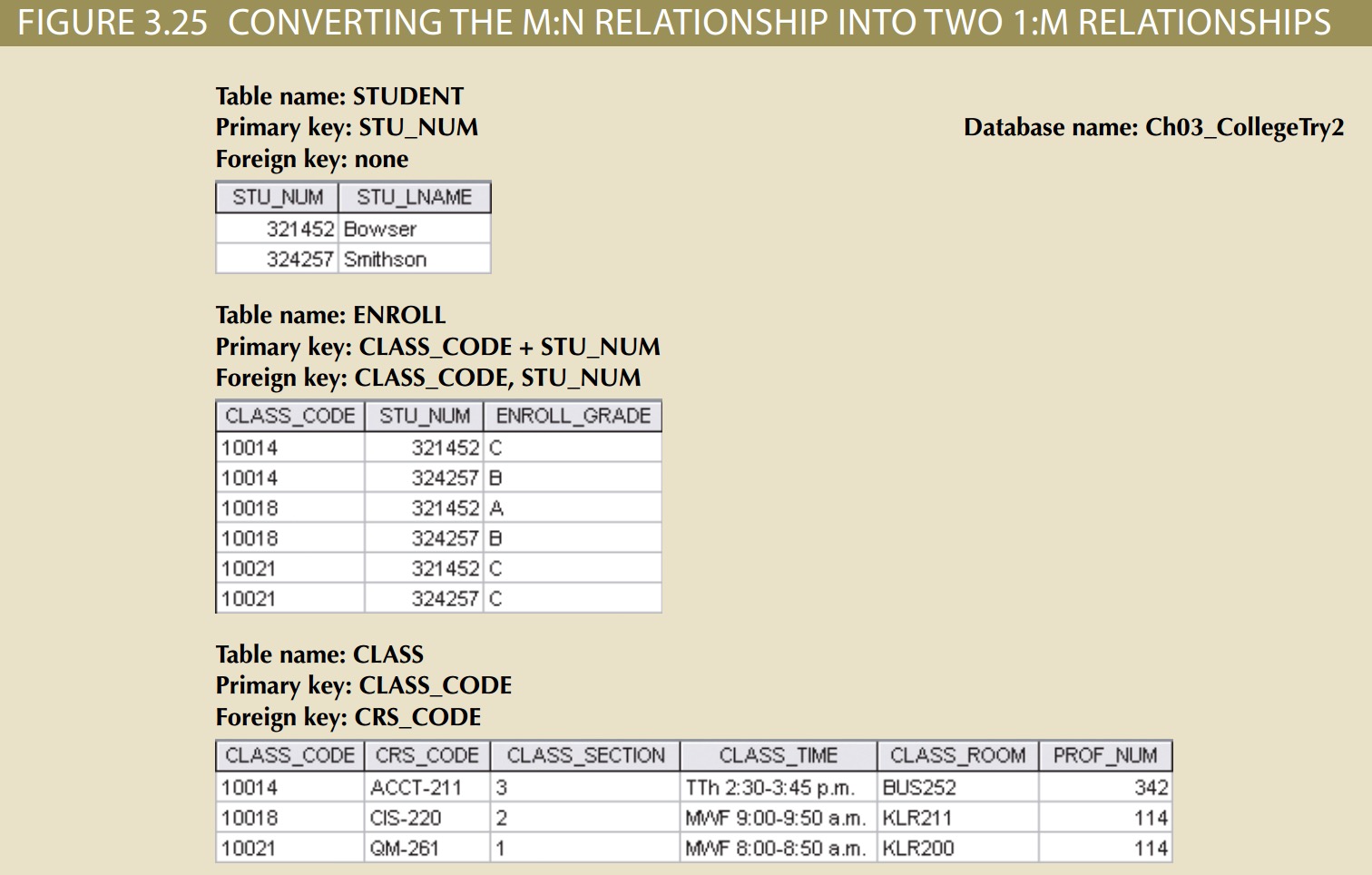
Because the ENROLL table in Figure 3.25 links two tables, STUDENT and CLASS, it is also called a linking table. In other words, a linking table is the implementation of a composite entity.
Data Redundency
The real test of redundancy is not how many copies of a given attribute are stored, but. whether the elimination of an attribute will eliminate information. Therefore, if you delete an attribute and the original information can still be generated through relational algebra, the inclusion of that attribute would be redundant.
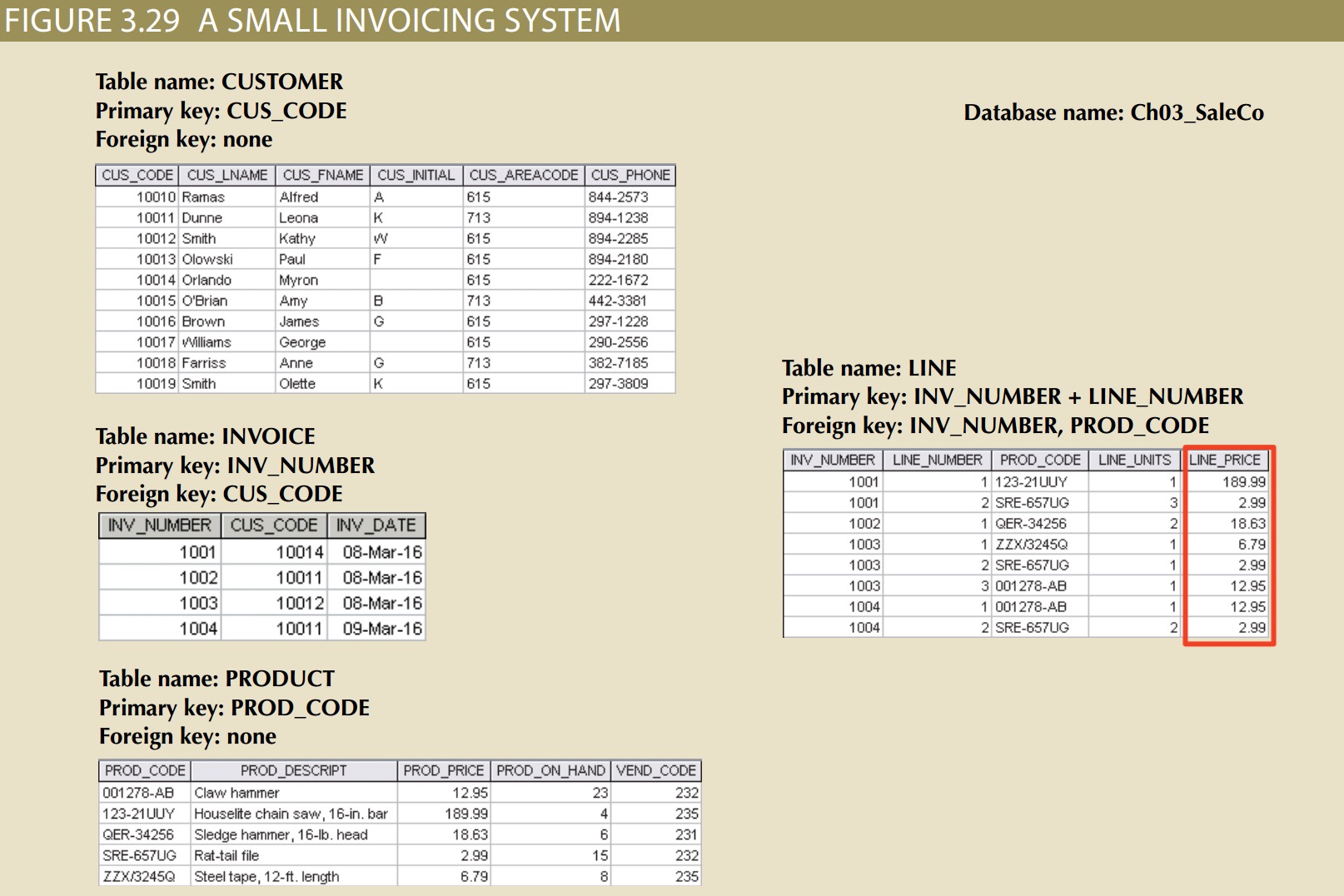
why does that same product price(Line_price) occur again in the LINE table? Is that not a data redundancy? It certainly appears to be, but this time, the apparent redundancy is crucial to the system’s success. Copying the product price from the PRODUCT table to the LINE table maintains the historical accuracy of the transactions. Suppose, for instance, that you fail to write the LINE_PRICE in the LINE table and that you use the PROD_PRICE from the PRODUCT table to calculate the sales revenue. Now suppose that the PRODUCT table’s PROD_PRICE changes, as prices frequently do. This price change will be properly reflected in all subsequent sales revenue calculations.
This kind of redundancy is necessary.
index
An index is an orderly arrangement used to logically access rows in a table. The index key is, in effect, the index’s reference point. Indexes play an important role in DBMSs for the implementation of primary keys.
When you define a table’s primary key, the DBMS automatically creates a unique index on the primary key column(s) you declared.
In a unique index, as its name implies, the index key can have only one pointer value (row) associated with it.
Codd’s Relational Database Rules
Bear in mind that even the dominant database vendors do not fully support all 12 rules.
Rule 1: Information Rule
The data stored in a database, may it be user data or metadata, must be a value of some table cell. Everything in a database must be stored in a table format.
Rule 2: Guaranteed Access Rule
Every single data element (value) is guaranteed to be accessible logically with a combination of table-name, primary-key (row value), and attribute-name (column value). No other means, such as pointers, can be used to access data.
Rule 3: Systematic Treatment of NULL Values
The NULL values in a database must be given a systematic and uniform treatment. This is a very important rule because a NULL can be interpreted as one the following − data is missing, data is not known, or data is not applicable.
Rule 4: Active Online Catalog
The structure description of the entire database must be stored in an online catalog, known as data dictionary, which can be accessed by authorized users. Users can use the same query language to access the catalog which they use to access the database itself.
Rule 5: Comprehensive Data Sub-Language Rule
A database can only be accessed using a language having linear syntax that supports data definition, data manipulation, and transaction management operations. This language can be used directly or by means of some application. If the database allows access to data without any help of this language, then it is considered as a violation.
Rule 6: View Updating Rule
All the views of a database, which can theoretically be updated, must also be updatable by the system.
Rule 7: High-Level Insert, Update, and Delete Rule
A database must support high-level insertion, updation, and deletion. This must not be limited to a single row, that is, it must also support union, intersection and minus operations to yield sets of data records.
Rule 8: Physical Data Independence
The data stored in a database must be independent of the applications that access the database. Any change in the physical structure of a database must not have any impact on how the data is being accessed by external applications.
Rule 9: Logical Data Independence
The logical data in a database must be independent of its user’s view (application). Any change in logical data must not affect the applications using it. For example, if two tables are merged or one is split into two different tables, there should be no impact or change on the user application. This is one of the most difficult rule to apply.
Rule 10: Integrity Independence
A database must be independent of the application that uses it. All its integrity constraints can be independently modified without the need of any change in the application. This rule makes a database independent of the front-end application and its interface.
Rule 11: Distribution Independence
The end-user must not be able to see that the data is distributed over various locations. Users should always get the impression that the data is located at one site only. This rule has been regarded as the foundation of distributed database systems.
Rule 12: Non-Subversion Rule
If a system has an interface that provides access to low-level records, then the interface must not be able to subvert the system and bypass security and integrity constraints.